How To Change The Color Of A Cell Based On Another Cells That Has A Symbol

Lesson 24: Conditional Formatting

/en/excel/charts/content/

Introduction

Let'southward say you lot have a worksheet with thousands of rows of data. It would be extremely hard to see patterns and trends just from examining the raw information. Similar to charts and sparklines, conditional formatting provides a way to visualize information and brand worksheets easier to sympathise.

Optional: Download our practise workbook.

Scout the video below to larn more about conditional formatting in Excel.

Understanding provisional formatting

Conditional formatting allows yous to automatically apply formatting—such as colors, icons, and data bars—to 1 or more cells based on the cell value. To do this, you'll need to create a conditional formatting rule. For example, a conditional formatting rule might exist: If the value is less than $2000, colour the cell red. By applying this rule, you'd be able to quickly run into which cells contain values less than $2000.

Conditional Formatting in Excel

To create a conditional formatting rule:

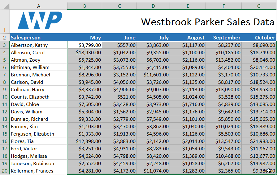
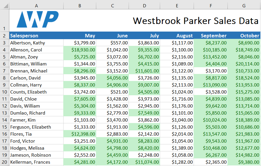
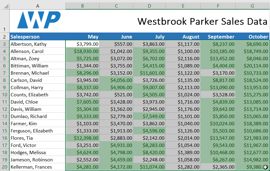
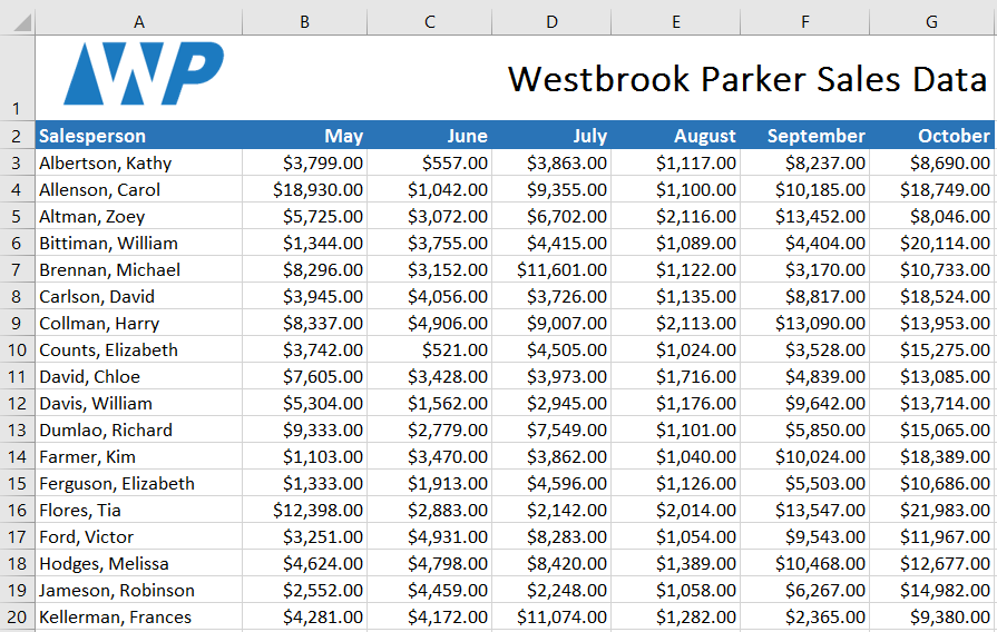
In our case, we have a worksheet containing sales data, and we'd like to encounter which salespeople are coming together their monthly sales goals. The sales goal is $4000 per month, so we'll create a conditional formatting dominion for whatsoever cells containing a value college than 4000.

Select the desired cells for the conditional formatting dominion.
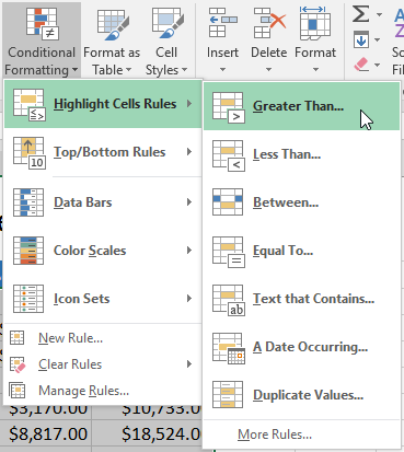
From the Abode tab, click the Conditional Formatting command. A drop-down menu volition appear.
Hover the mouse over the desired conditional formatting type, then select the desired rule from the menu that appears. In our example, we want to highlight cells that are greater than $4000.
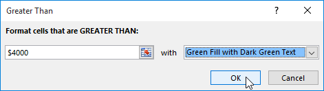
A dialog box will announced. Enter the desired value(south) into the blank field. In our example, nosotros'll enter 4000 as our value.
Select a formatting way from the drop-down card. In our example, we'll choose Green Fill with Dark Green Text, so click OK.
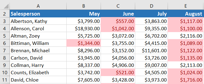
The conditional formatting will be applied to the selected cells. In our example, it'southward easy to run into which salespeople reached the $4000 sales goal for each calendar month.

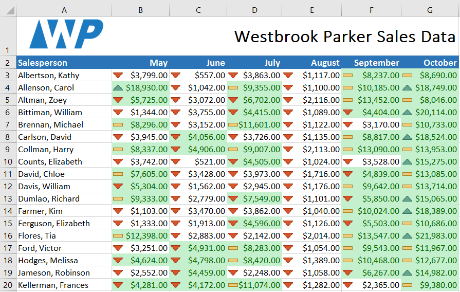
You tin employ multiple provisional formatting rules to a prison cell range or worksheet, allowing you to visualize different trends and patterns in your data.

Multiple conditional formatting rules on the same area of a worksheet

Conditional formatting presets

Excel has several predefined styles—or presets—you can utilise to rapidly apply conditional formatting to your data. They are grouped into three categories:

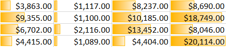
Data Bars are horizontal confined added to each jail cell, much like a bar graph.
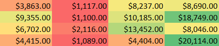
Color Scales modify the color of each cell based on its value. Each colour scale uses a two- or three-color slope. For example, in the Green-Yellow-Red colour scale, the highest values are greenish, the average values are yellow, and the lowest values are red.
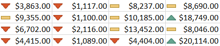
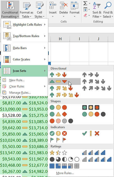
Icon Sets add a specific icon to each cell based on its value.

To use preset conditional formatting:

Select the desired cells for the conditional formatting dominion.
Click the Provisional Formatting control. A drib-downwards menu will appear.
Hover the mouse over the desired preset, then choose a preset style from the menu that appears.
The conditional formatting will be practical to the selected cells.

Removing provisional formatting

To remove conditional formatting:

Click the Conditional Formatting control. A drop-downwardly menu will announced.
Hover the mouse over Clear Rules, and so cull which rules you lot want to clear. In our example, we'll select Clear Rules from Entire Canvas to remove all conditional formatting from the worksheet.
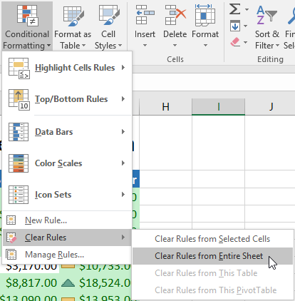
The conditional formatting will be removed.

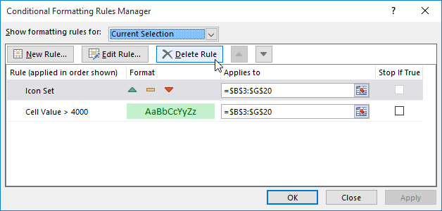
Click Manage Rules to edit or delete private rules. This is especially useful if y'all've practical multiple rules to a worksheet.

The Conditional Formatting Rules Manager

Challenge!

Open up our practice workbook.
Click the Challenge worksheet tab in the lesser-left of the workbook.
Select cells B3:J17.
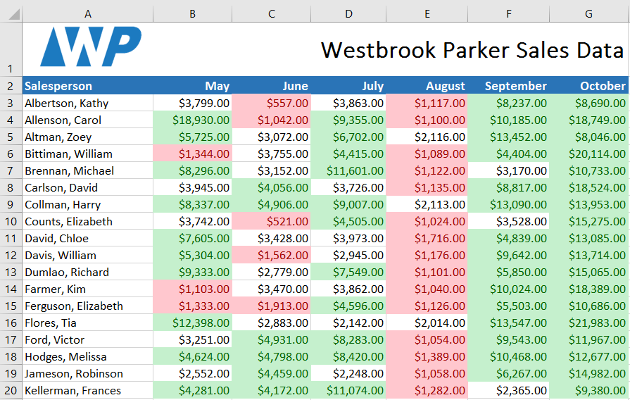
Let'southward say you're the teacher and desire to easily see all of the grades that are below passing. Apply Provisional Formatting so it Highlights Cells containing values Less Than 70 with a light ruby-red fill.
At present y'all desire to see how the grades compare to each other. Nether the Conditional Formatting tab, select the Icon Set up called three Symbols (Circled). Hint: The names of the icon sets will announced when you hover over them.
Your spreadsheet should expect like this:
Using the Manage Rules feature, remove the lite cherry fill, just keep the icon fix.